如果最小二乘線性回歸算法最小化到回歸直線的豎直距離（即，平行于y軸方向），則戴明回歸最小化到回歸直線的總距離（即，垂直于回歸直線）。其最小化x值和y值兩個方向的誤差，具體的對比圖如下圖。

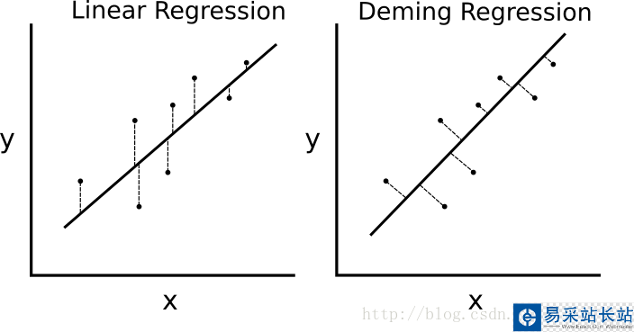
線性回歸算法和戴明回歸算法的區(qū)別。左邊的線性回歸最小化到回歸直線的豎直距離；右邊的戴明回歸最小化到回歸直線的總距離。

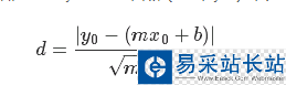
線性回歸算法的損失函數(shù)最小化豎直距離；而這里需要最小化總距離。給定直線的斜率和截距，則求解一個點(diǎn)到直線的垂直距離有已知的幾何公式。代入幾何公式并使TensorFlow最小化距離。

損失函數(shù)是由分子和分母組成的幾何公式。給定直線y=mx+b，點(diǎn)（x0，y0），則求兩者間的距離的公式為：

# 戴明回歸#----------------------------------## This function shows how to use TensorFlow to# solve linear Deming regression.# y = Ax + b## We will use the iris data, specifically:# y = Sepal Length# x = Petal Widthimport matplotlib.pyplot as pltimport numpy as npimport tensorflow as tffrom sklearn import datasetsfrom tensorflow.python.framework import opsops.reset_default_graph()# Create graphsess = tf.Session()# Load the data# iris.data = [(Sepal Length, Sepal Width, Petal Length, Petal Width)]iris = datasets.load_iris()x_vals = np.array([x[3] for x in iris.data])y_vals = np.array([y[0] for y in iris.data])# Declare batch sizebatch_size = 50# Initialize placeholdersx_data = tf.placeholder(shape=[None, 1], dtype=tf.float32)y_target = tf.placeholder(shape=[None, 1], dtype=tf.float32)# Create variables for linear regressionA = tf.Variable(tf.random_normal(shape=[1,1]))b = tf.Variable(tf.random_normal(shape=[1,1]))# Declare model operationsmodel_output = tf.add(tf.matmul(x_data, A), b)# Declare Demming loss functiondemming_numerator = tf.abs(tf.subtract(y_target, tf.add(tf.matmul(x_data, A), b)))demming_denominator = tf.sqrt(tf.add(tf.square(A),1))loss = tf.reduce_mean(tf.truediv(demming_numerator, demming_denominator))# Declare optimizermy_opt = tf.train.GradientDescentOptimizer(0.1)train_step = my_opt.minimize(loss)# Initialize variablesinit = tf.global_variables_initializer()sess.run(init)# Training looploss_vec = []for i in range(250):  rand_index = np.random.choice(len(x_vals), size=batch_size)  rand_x = np.transpose([x_vals[rand_index]])  rand_y = np.transpose([y_vals[rand_index]])  sess.run(train_step, feed_dict={x_data: rand_x, y_target: rand_y})  temp_loss = sess.run(loss, feed_dict={x_data: rand_x, y_target: rand_y})  loss_vec.append(temp_loss)  if (i+1)%50==0:    print('Step #' + str(i+1) + ' A = ' + str(sess.run(A)) + ' b = ' + str(sess.run(b)))    print('Loss = ' + str(temp_loss))# Get the optimal coefficients[slope] = sess.run(A)[y_intercept] = sess.run(b)# Get best fit linebest_fit = []for i in x_vals: best_fit.append(slope*i+y_intercept)# Plot the resultplt.plot(x_vals, y_vals, 'o', label='Data Points')plt.plot(x_vals, best_fit, 'r-', label='Best fit line', linewidth=3)plt.legend(loc='upper left')plt.title('Sepal Length vs Pedal Width')plt.xlabel('Pedal Width')plt.ylabel('Sepal Length')plt.show()# Plot loss over timeplt.plot(loss_vec, 'k-')plt.title('L2 Loss per Generation')plt.xlabel('Generation')plt.ylabel('L2 Loss')plt.show()