也有些正則方法可以限制回歸算法輸出結果中系數的影響,其中最常用的兩種正則方法是lasso回歸和嶺回歸。
lasso回歸和嶺回歸算法跟常規線性回歸算法極其相似,有一點不同的是,在公式中增加正則項來限制斜率(或者凈斜率)。這樣做的主要原因是限制特征對因變量的影響,通過增加一個依賴斜率A的損失函數實現。
對于lasso回歸算法,在損失函數上增加一項:斜率A的某個給定倍數。我們使用TensorFlow的邏輯操作,但沒有這些操作相關的梯度,而是使用階躍函數的連續估計,也稱作連續階躍函數,其會在截止點跳躍擴大。一會就可以看到如何使用lasso回歸算法。
對于嶺回歸算法,增加一個L2范數,即斜率系數的L2正則。
# LASSO and Ridge Regression# lasso回歸和嶺回歸# # This function shows how to use TensorFlow to solve LASSO or # Ridge regression for # y = Ax + b# # We will use the iris data, specifically: # y = Sepal Length # x = Petal Width# import required librariesimport matplotlib.pyplot as pltimport sysimport numpy as npimport tensorflow as tffrom sklearn import datasetsfrom tensorflow.python.framework import ops# Specify 'Ridge' or 'LASSO'regression_type = 'LASSO'# clear out old graphops.reset_default_graph()# Create graphsess = tf.Session()#### Load iris data#### iris.data = [(Sepal Length, Sepal Width, Petal Length, Petal Width)]iris = datasets.load_iris()x_vals = np.array([x[3] for x in iris.data])y_vals = np.array([y[0] for y in iris.data])#### Model Parameters#### Declare batch sizebatch_size = 50# Initialize placeholdersx_data = tf.placeholder(shape=[None, 1], dtype=tf.float32)y_target = tf.placeholder(shape=[None, 1], dtype=tf.float32)# make results reproducibleseed = 13np.random.seed(seed)tf.set_random_seed(seed)# Create variables for linear regressionA = tf.Variable(tf.random_normal(shape=[1,1]))b = tf.Variable(tf.random_normal(shape=[1,1]))# Declare model operationsmodel_output = tf.add(tf.matmul(x_data, A), b)#### Loss Functions#### Select appropriate loss function based on regression typeif regression_type == 'LASSO': # Declare Lasso loss function # 增加損失函數,其為改良過的連續階躍函數,lasso回歸的截止點設為0.9。 # 這意味著限制斜率系數不超過0.9 # Lasso Loss = L2_Loss + heavyside_step, # Where heavyside_step ~ 0 if A < constant, otherwise ~ 99 lasso_param = tf.constant(0.9) heavyside_step = tf.truediv(1., tf.add(1., tf.exp(tf.multiply(-50., tf.subtract(A, lasso_param))))) regularization_param = tf.multiply(heavyside_step, 99.) loss = tf.add(tf.reduce_mean(tf.square(y_target - model_output)), regularization_param)elif regression_type == 'Ridge': # Declare the Ridge loss function # Ridge loss = L2_loss + L2 norm of slope ridge_param = tf.constant(1.) ridge_loss = tf.reduce_mean(tf.square(A)) loss = tf.expand_dims(tf.add(tf.reduce_mean(tf.square(y_target - model_output)), tf.multiply(ridge_param, ridge_loss)), 0)else: print('Invalid regression_type parameter value',file=sys.stderr)#### Optimizer#### Declare optimizermy_opt = tf.train.GradientDescentOptimizer(0.001)train_step = my_opt.minimize(loss)#### Run regression#### Initialize variablesinit = tf.global_variables_initializer()sess.run(init)# Training looploss_vec = []for i in range(1500): rand_index = np.random.choice(len(x_vals), size=batch_size) rand_x = np.transpose([x_vals[rand_index]]) rand_y = np.transpose([y_vals[rand_index]]) sess.run(train_step, feed_dict={x_data: rand_x, y_target: rand_y}) temp_loss = sess.run(loss, feed_dict={x_data: rand_x, y_target: rand_y}) loss_vec.append(temp_loss[0]) if (i+1)%300==0: print('Step #' + str(i+1) + ' A = ' + str(sess.run(A)) + ' b = ' + str(sess.run(b))) print('Loss = ' + str(temp_loss)) print('/n')#### Extract regression results#### Get the optimal coefficients[slope] = sess.run(A)[y_intercept] = sess.run(b)# Get best fit linebest_fit = []for i in x_vals: best_fit.append(slope*i+y_intercept)#### Plot results#### Plot regression line against data pointsplt.plot(x_vals, y_vals, 'o', label='Data Points')plt.plot(x_vals, best_fit, 'r-', label='Best fit line', linewidth=3)plt.legend(loc='upper left')plt.title('Sepal Length vs Pedal Width')plt.xlabel('Pedal Width')plt.ylabel('Sepal Length')plt.show()# Plot loss over timeplt.plot(loss_vec, 'k-')plt.title(regression_type + ' Loss per Generation')plt.xlabel('Generation')plt.ylabel('Loss')plt.show()
新聞熱點


疑難解答