python有專門的神經(jīng)網(wǎng)絡(luò)庫,但為了加深印象,我自己在numpy庫的基礎(chǔ)上,自己編寫了一個簡單的神經(jīng)網(wǎng)絡(luò)程序,是基于Rosenblatt感知器的,這個感知器建立在一個線性神經(jīng)元之上,神經(jīng)元模型的求和節(jié)點(diǎn)計算作用于突觸輸入的線性組合,同時結(jié)合外部作用的偏置,對若干個突觸的輸入求和后進(jìn)行調(diào)節(jié)。為了便于觀察,這里的數(shù)據(jù)采用二維數(shù)據(jù)。
目標(biāo)函數(shù)是訓(xùn)練結(jié)果的誤差的平方和,由于目標(biāo)函數(shù)是一個二次函數(shù),只存在一個全局極小值,所以采用梯度下降法的策略尋找目標(biāo)函數(shù)的最小值。
代碼如下:
import numpy as np import pylab as pl b=1 #偏置 a=0.3 #學(xué)習(xí)率 x=np.array([[b,1,3],[b,2,3],[b,1,8],[b,2,15],[b,3,7],[b,4,29],[b,4,8],[b,4,20]]) #訓(xùn)練數(shù)據(jù) d=np.array([1,1,-1,-1,1,-1,1,-1]) #訓(xùn)練數(shù)據(jù)類別 w=np.array([b,0,0]) #初始w def sgn(v): if v>=0: return 1 else: return -1 def comy(myw,myx): return sgn(np.dot(myw.T,myx)) def neww(oldw,myd,myx,a): return oldw+a*(myd-comy(oldw,myx))*myx for ii in range(5): #迭代次數(shù) i=0 for xn in x: w=neww(w,d[i],xn,a) i+=1 print w myx=x[:,1] #繪制訓(xùn)練數(shù)據(jù) myy=x[:,2] pl.subplot(111) x_max=np.max(myx)+15 x_min=np.min(myx)-5 y_max=np.max(myy)+50 y_min=np.min(myy)-5 pl.xlabel(u"x") pl.xlim(x_min,x_max) pl.ylabel(u"y") pl.ylim(y_min,y_max) for i in range(0,len(d)): if d[i]==1: pl.plot(myx[i],myy[i],'r*') else: pl.plot(myx[i],myy[i],'ro') #繪制測試點(diǎn) test=np.array([b,9,19]) if comy(w,test)>0: pl.plot(test[1],test[2],'b*') else: pl.plot(test[1],test[2],'bo') test=np.array([b,9,64]) if comy(w,test)>0: pl.plot(test[1],test[2],'b*') else: pl.plot(test[1],test[2],'bo') test=np.array([b,9,16]) if comy(w,test)>0: pl.plot(test[1],test[2],'b*') else: pl.plot(test[1],test[2],'bo') test=np.array([b,9,60]) if comy(w,test)>0: pl.plot(test[1],test[2],'b*') else: pl.plot(test[1],test[2],'bo') #繪制分類線 testx=np.array(range(0,20)) testy=testx*2+1.68 pl.plot(testx,testy,'g--') pl.show() for xn in x: print "%d %d => %d" %(xn[1],xn[2],comy(w,xn))
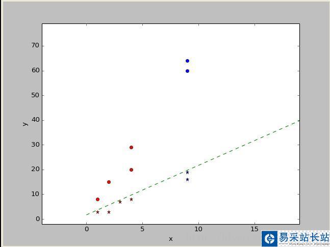
圖中紅色是訓(xùn)練數(shù)據(jù),藍(lán)色是測試數(shù)據(jù),圓點(diǎn)代表類別-1.星點(diǎn)代表類別1。由圖可知,對于線性可分的數(shù)據(jù)集,Rosenblatt感知器的分類效果還是不錯的。
以上就是本文的全部內(nèi)容,希望對大家的學(xué)習(xí)有所幫助,也希望大家多多支持武林站長站。
新聞熱點(diǎn)


疑難解答
圖片精選